

As I was browsing through topics to write about, I came across an article on predictive microbiological modelling developed for botulism prediction. Albeit lesser known, and usually not discussed widely, predictive modelling has been used in various fields – from election results and climatic events to deep learning and email spam detection. As such, I decided to write a short article explaining predictive microbiology and its current use in the food industry.
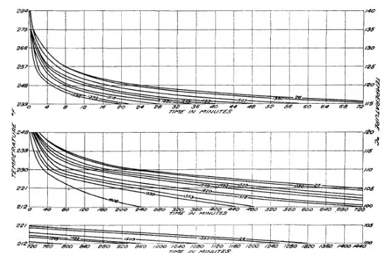
In predictive microbiology, a simplified approach is taken to measure microbial responses under defined parameters, which is then expressed in a mathematical equation. Using the same, one can predict responses to a different set of conditions, that was not included in the original testing. Historically, the first proposed model was the classical log-linear model of bacterial inactivation by heat shown in Fig 1 (Bigelow & Esty, 1920), which was followed by several other bacterial growth kinetic models – Arrhenius model, cardinal temperature model, and gamma concept model etc. Using these, one can predict bacterial growth, inactivation or death, metabolite or toxin production to also finding the absolute limits for several microbes in food environments.
To begin with, we will define some parameters that’s common use in predictive modelling. Generally speaking, a model can be built in the following way.
Input parameters -> Function or Relation -> Output response
Or the mathematical function explaining the above can be expressed in a linear function as
Y= αX1 + βX2 + γX3 + ε
where Y is the dependent variable or the output response, (X1 X2 X3 ) are the independent variables or the input parameters, (αβγ) are the regression coefficients which explain the functional relationship between the variables and ε is the error. Another case would be a non-linear model, expressed as
Y= e αX + ε
Which is mostly used in predictive microbiology to describe concentration change over time, or other physical processes such as microbial transfer, metabolite production etc. As we translate these ideas into food safety principles, food scientists often use a risk-based approach called quantitative microbial risk assessment (QMRA) to identify hazards and controls. The process involves characterizing a risk (pathogen) both quantitatively and qualitatively, in various combinations to eliminate the associated uncertainty in achieving a safe product. Now we will look at various kinds of primary, and secondary models explaining the kinetics and few examples for each.
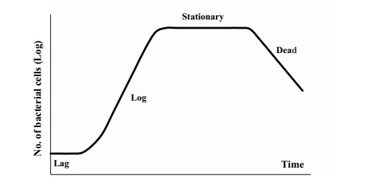
Primary models: Estimates the growth kinetics as a function of time. Usually, it describes microbial concentration increase or decrease over time due to extrinsic or intrinsic factors (Fig 1), and the obtained results are only applicable under the same conditions considered during the model building. The famous bacterial growth curve with lag, exponential, stationary and death phase is an example of the primary model (Fig 2). One may wonder, where do primary model finds their use? These primary models are used extensively in developing high-temperature kill treatments for spore-forming bacteria and sterilization techniques (UHT, HTST etc).
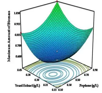
Now that we know what primary models are, let’s move on to secondary modelling. Generally, secondary models arise when you want to describe the relationship between several factors, say water activity, temperature, pH, salt concentration etc. on the final outcome or dependent variable. One example is the response-surface methodology, which are secondary models, where polynomial equations of various orders are used, and usually expressed as contour plots (2D) or surface plots (3D; Fig 3). The correlation coefficient (R2) is obtained for each model, and higher the value, better the fit of the model. An important benefit of using such models is that one can easily optimize any food formulations to achieve the combination of factors that will inhibit or grow the microbes.
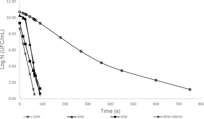
As we continue exploring, one can also use several software tools that can be used for modelling; Examples include Matlab, MiniTab, GInaFit, MicroHibro among many others. GInaFit, Matlab, and Minitab have an excel component, where users can input data, and select a model to run the equation, which results in an output tab with necessary data fitting performed. Closer to home, MLA (Meat and Livestock Australia) has an E. coli inactivation model tool that allows manufacturers to assess their fermenting conditions and their efficacy in killing E. coli. Jessica et al (2019) have developed a predictive model for Salmonella inactivation in infant formula using microwave processing. The researchers selected five distinct Salmonella strains, which were later subjected to heat inactivation treatment using microwave heating. Bacterial enumeration was performed in intervals, and different survival models (Log-linear, Biphasic, Square root models) were constructed using GinaFit, and logCFU/mL graphs were plotted against time (Fig 4). As discussed earlier, R2 (correlation coefficient) and error was calculated (R2 = 0.98), and model validation was performed by calculating the predictive efficacy. This has serious food safety implications, as Salmonella infections causing diarrheal diseases account for almost one quarter of all the cases in the world. While we work towards global food safety, developing countries with limited resources can implement such food processing techniques that are available firsthand to alleviate their risks.
Another real-world use of predictive modelling can be seen in global supply chain, where one can employ predictive models to monitor intrinsic and extrinsic factors, and effectively maximising the shelf-life and preventing any food safety incidents. As technology advances in an ever-increasing rate, sensors can provide real-time data to integrated predictive models, by monitoring food safety variables. Tamplin (2018) discusses how food quality and safety can be monitored , and reports on several predictive models developed for supply chain management. One such example is the Vibrio bacterium models for oysters – where the variables include seawater surface temperature, harvesting season, region, and water activity. As a model is developed, companies can investigate different scenarios and excersise their control strategies in each step of their supply chain to minimize food spoilage and improve safety. One can build a primary model and others can build upon it for different foods, targetting a myriad of microbes, ultimately providing better food safety for everyone.
Although incredibly useful, there are some limitations to predictive modelling. Most models are developed on the assumption that microbial responses are predictable and consistent, and any inconsistencies associated with the responses are at times designated and analysed as errors and output variations during verification. Consequently, cross validation is crucial when using your model to make food safety decisions, as validity shrinkage – a term refering to predictive modelling’s validity reduction when you take a sample from a different population other than the sample used originally to develop the model – should be accounted for, and one should make sure to incorporate this to maximise the model’s accuracy during testing. Increase the sample size, and collect data from varied population, and incorporate prior studies that may provide specific knowledge on your parameters and variables. As such, be wary of using one too many parameters, as it may result in multicollinearity – a condition where independent variables seemingly depend on each other which weakens the statistical significance, as variables need to be distinct and independent during modelling.
References
Bigelow, W. D, & Esty, J. R. (1920). The Thermal Death Point in Relation to Time of Typical Thermophilic Organisms. The Journal of Infectious Diseases, 27(6), 602–617. https://doi.org/10.1093/infdis/27.6.602
Jéssica B. Portela, Pablo T. Coimbra, Leandro P. Cappato, Verônica O. Alvarenga, Rodrigo B.A. Oliveira, Karen S. Pereira, Denise R.P. Azeredo, Anderson S. Sant’Ana, Janaina S. Nascimento, Adriano G. Cruz, Predictive model for inactivation of salmonella in infant formula during microwave heating processing, Food Control, Volume 104, 2019, Pages 308-312, ISSN 0956-7135, https://doi.org/10.1016/j.foodcont.2019.05.006.
Mark L. Tamplin, Integrating predictive models and sensors to manage food stability in supply chains, Food Microbiology, Volume 75, 2018, Pages 90-94, ISSN 0740-0020, https://doi.org/10.1016/j.fm.2017.12.001.
